This document demonstrates how to perform Principal Component Analysis (PCA) in Python using the scikit-learn library. PCA is a dimensionality reduction technique that transforms a set of possibly correlated variables into a set of linearly uncorrelated variables called principal components. We will use the adult_income_dataset.csv for this demonstration.
2 Load Data
First, we load the necessary libraries and the income dataset.
Code
import pandas as pdfrom sklearn.preprocessing import StandardScalerfrom sklearn.decomposition import PCAimport matplotlib.pyplot as pltimport seaborn as sns# Load the income datasetincome_df = pd.read_csv("../data/adult_income_dataset.csv")
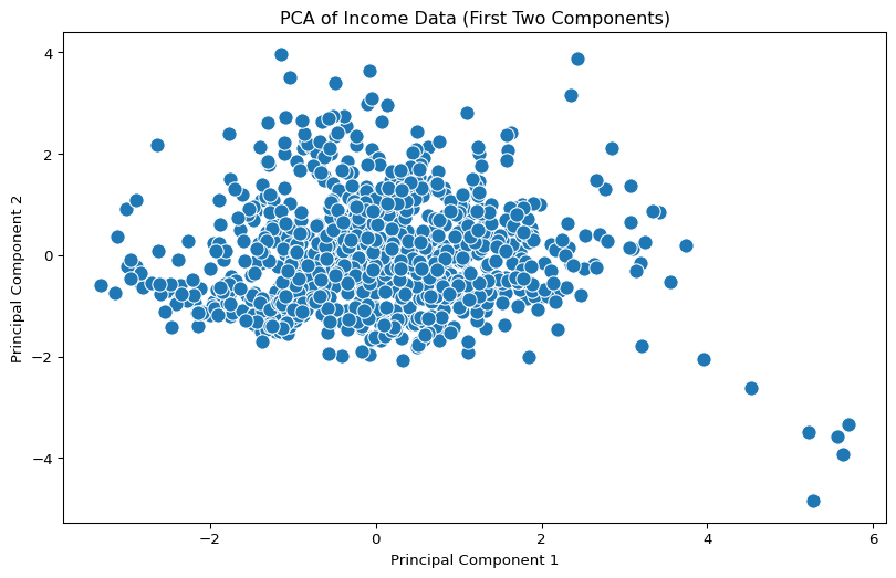
We can visualize the data projected onto the first two principal components.
Code
pca_2d = PCA(n_components=2)principal_components_2d = pca_2d.fit_transform(scaled_income)principal_df_2d = pd.DataFrame(data = principal_components_2d, columns = ['principal component 1', 'principal component 2'])plt.figure(figsize=(10, 6))sns.scatterplot(x='principal component 1', y='principal component 2', data=principal_df_2d, palette='viridis', s=100)plt.title('PCA of Income Data (First Two Components)')plt.xlabel('Principal Component 1')plt.ylabel('Principal Component 2')plt.show()
5 Conclusion
This document provided an overview of Principal Component Analysis in Python using scikit-learn. We demonstrated how to perform PCA on the income dataset and visualize the results.
6 Keeping Top 5 Components
We can select and work with a reduced number of principal components, for example, the top 5 components that explain a significant portion of the variance.
Code
pca_5 = PCA(n_components=5)principal_components_5 = pca_5.fit_transform(scaled_income)print("Shape of data after keeping top 5 components:", principal_components_5.shape)print("First 5 rows of the top 5 principal components:\n", principal_components_5[:5])# Explained variance by the top 5 componentsprint("Explained variance ratio of top 5 components:", pca_5.explained_variance_ratio_)print("Cumulative explained variance of top 5 components:", pca_5.explained_variance_ratio_.cumsum()[-1])
Shape of data after keeping top 5 components: (1000, 5)
First 5 rows of the top 5 principal components:
[[-0.66259976 -0.6901712 -0.12605474 -0.50941084 0.03776418]
[ 0.20225145 0.96781646 -0.85529215 -0.86061386 0.21421535]
[ 1.04905925 -1.10717674 0.30121431 -0.15852958 0.92758685]
[ 0.05573208 -1.37283113 0.10129154 -0.58123139 -0.12323307]
[ 0.11670067 -0.64810635 0.06004221 0.06858625 0.82368069]]
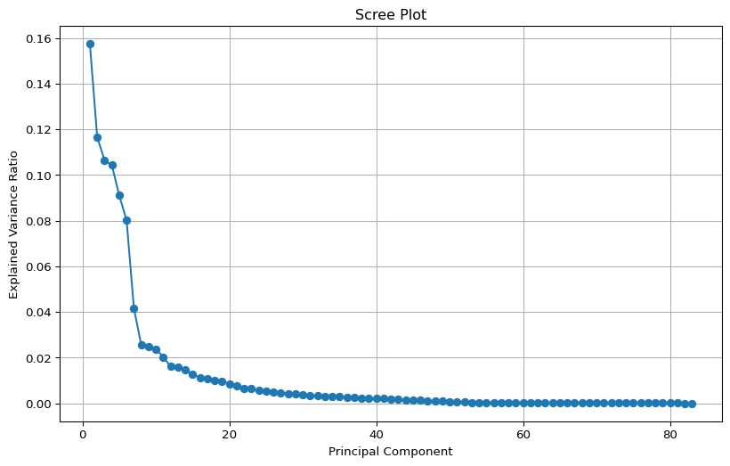
Explained variance ratio of top 5 components: [0.15732576 0.11650394 0.10643612 0.10423658 0.09096257]
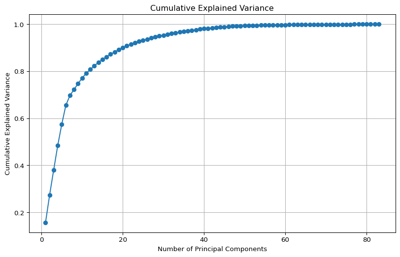
Cumulative explained variance of top 5 components: 0.575464968553261
Source Code
---title: "PCA: Income Data with Python"subtitle: "Using sklearn"execute: warning: false error: falseformat: html: toc: true toc-location: right code-fold: show code-tools: true number-sections: true code-block-bg: true code-block-border-left: "#31BAE9"---## IntroductionThis document demonstrates how to perform Principal Component Analysis (PCA) in Python using the `scikit-learn` library. PCA is a dimensionality reduction technique that transforms a set of possibly correlated variables into a set of linearly uncorrelated variables called principal components. We will use the `adult_income_dataset.csv` for this demonstration.## Load DataFirst, we load the necessary libraries and the income dataset.```{python}#| label: load-data#| echo: trueimport pandas as pdfrom sklearn.preprocessing import StandardScalerfrom sklearn.decomposition import PCAimport matplotlib.pyplot as pltimport seaborn as sns# Load the income datasetincome_df = pd.read_csv("../data/adult_income_dataset.csv")``````{python}# Handle missing values and sample dataincome_df_clean = income_df.drop('income', axis=1).dropna().sample(n=1000, random_state=42)# Separate numerical and categorical columnsnumerical_cols = income_df_clean.select_dtypes(include=['int64', 'float64']).columnscategorical_cols = income_df_clean.select_dtypes(include=['object']).columns# One-hot encode categorical featuresincome_df_encoded = pd.get_dummies(income_df_clean, columns=categorical_cols, drop_first=True)# Standardize numerical featuresscaler = StandardScaler()income_df_encoded[numerical_cols] = scaler.fit_transform(income_df_encoded[numerical_cols])scaled_income = income_df_encoded.values```## Principal Component AnalysisWe will perform PCA on the preprocessed income data.```{python}#| label: pca#| echo: truepca = PCA()pca.fit(scaled_income)# Explained variance ratioexplained_variance_ratio = pca.explained_variance_ratio_# Scree plotplt.figure(figsize=(10, 6))plt.plot(range(1, len(explained_variance_ratio) +1), explained_variance_ratio, marker='o')plt.title('Scree Plot')plt.xlabel('Principal Component')plt.ylabel('Explained Variance Ratio')plt.grid(True)plt.show()# Cumulative explained variancecumulative_explained_variance = explained_variance_ratio.cumsum()plt.figure(figsize=(10, 6))plt.plot(range(1, len(cumulative_explained_variance) +1), cumulative_explained_variance, marker='o')plt.title('Cumulative Explained Variance')plt.xlabel('Number of Principal Components')plt.ylabel('Cumulative Explained Variance')plt.grid(True)plt.show()```## PCA Results VisualizationWe can visualize the data projected onto the first two principal components.```{python}#| label: pca-viz#| echo: truepca_2d = PCA(n_components=2)principal_components_2d = pca_2d.fit_transform(scaled_income)principal_df_2d = pd.DataFrame(data = principal_components_2d, columns = ['principal component 1', 'principal component 2'])plt.figure(figsize=(10, 6))sns.scatterplot(x='principal component 1', y='principal component 2', data=principal_df_2d, palette='viridis', s=100)plt.title('PCA of Income Data (First Two Components)')plt.xlabel('Principal Component 1')plt.ylabel('Principal Component 2')plt.show()```## ConclusionThis document provided an overview of Principal Component Analysis in Python using `scikit-learn`. We demonstrated how to perform PCA on the income dataset and visualize the results.## Keeping Top 5 ComponentsWe can select and work with a reduced number of principal components, for example, the top 5 components that explain a significant portion of the variance.```{python}#| label: top-5-components-python#| echo: truepca_5 = PCA(n_components=5)principal_components_5 = pca_5.fit_transform(scaled_income)print("Shape of data after keeping top 5 components:", principal_components_5.shape)print("First 5 rows of the top 5 principal components:\n", principal_components_5[:5])# Explained variance by the top 5 componentsprint("Explained variance ratio of top 5 components:", pca_5.explained_variance_ratio_)print("Cumulative explained variance of top 5 components:", pca_5.explained_variance_ratio_.cumsum()[-1])```